
Kinematic equations are a set of mathematical equations that describe the motion of objects. These equations allow us to determine various properties of an object’s motion, such as its position, velocity, and acceleration, based on known information. In physics, understanding and applying these equations is crucial in solving problems related to kinematics.
A worksheet containing kinematic problems is a valuable tool for practicing and reinforcing the concepts and formulas involved in kinematics. Working through these problems not only helps students become more familiar with the equations but also develops their problem-solving skills and ability to apply physics principles to real-life situations.
In this article, we provide answers to a kinematic equations worksheet. By going through the solutions, students can verify their own answers, identify any mistakes or errors they may have made, and gain a better understanding of the concepts and calculations involved in kinematics.
What are Kinematic Equations?
Kinematic equations are a set of equations that describe the relationships between the displacement, velocity, acceleration, and time of an object in motion. These equations are derived from Newton’s laws of motion and are used to solve problems involving motion.
The four basic kinematic equations are:
- Displacement equation: Δx = v0t + (1/2)at2
- Velocity equation: v = v0 + at
- Acceleration equation: v2 = v02 + 2aΔx
- Time equation: Δx = (1/2)(v0 + v)t
These equations can be used to solve a variety of problems, such as finding the final velocity of an object given its initial velocity, acceleration, and displacement, or finding the displacement of an object given its initial velocity, acceleration, and time.
It is important to note that these equations only apply to objects moving with constant acceleration. If the acceleration is not constant, more complex equations or numerical methods may be required to solve the problem.
Definition of Kinematic Equations
Kinematic equations are a set of mathematical formulas used to describe the motion of objects in terms of their position, velocity, and acceleration. These equations are derived from the principles of classical mechanics and can be used to solve various problems related to motion.
The key variables in kinematic equations are:
- Position (x): The location of an object in space at a given time.
- Velocity (v): The rate of change of position with respect to time. It is a vector quantity, meaning it has both magnitude and direction.
- Acceleration (a): The rate of change of velocity with respect to time. It is also a vector quantity.
- Time (t): The duration of the motion or the interval between two events.
The kinematic equations relate these variables to one another and allow us to calculate unknown quantities when given enough information. There are four kinematic equations, which are:
- Position equation: x = x0 + v0t + 0.5at2
- Velocity equation: v = v0 + at
- Acceleration equation: v2 = v02 + 2a(x – x0)
- Displacement equation: x – x0 = 0.5(v + v0)t
These equations can be used to solve a wide range of problems, including finding the final position or velocity of an object, determining the time taken to reach a certain position, or calculating the acceleration of an object given its initial and final velocities.
Importance of Kinematic Equations in Physics
Kinematic equations are fundamental tools in the study of mechanics in physics. They describe the motion of objects and allow us to calculate various parameters related to their movement, such as displacement, velocity, and acceleration. Without these equations, it would be extremely challenging to analyze and understand the motion of objects in a precise and quantitative manner.
The first kinematic equation, s = ut + 1/2at^2, relates an object’s displacement (s) to its initial velocity (u), time (t), and acceleration (a). By rearranging the equation, we can determine any of these variables as long as we know the values of the others. This equation is particularly useful for calculating displacement when acceleration is constant.
The second kinematic equation, v = u + at, connects an object’s final velocity (v) with its initial velocity (u), acceleration (a), and time (t). This equation allows us to determine the final velocity of an object undergoing constant acceleration. It is often used to solve problems involving an object’s speed or change in velocity over time.
The third kinematic equation, s = (u + v)t/2, involves an object’s displacement (s), initial velocity (u), final velocity (v), and time (t). It provides a way to calculate displacement when the initial and final velocities are known, and allows us to analyze motion under non-uniform acceleration.
The fourth kinematic equation, v^2 = u^2 + 2as, connects an object’s final velocity (v) with its initial velocity (u), acceleration (a), and displacement (s). This equation is useful for calculating an object’s final velocity when its initial velocity, acceleration, and displacement are known. It also helps in understanding the relationship between velocity and displacement.
In summary, kinematic equations play a crucial role in physics by providing a mathematical framework for describing and analyzing the motion of objects. They allow us to make quantitative predictions about an object’s position, velocity, and acceleration, and help us better understand the fundamental principles underlying the behavior of physical systems.
Types of Kinematic Equations
The study of kinematics involves the analysis of motion and its various attributes such as displacement, velocity, and acceleration. To describe this motion mathematically, we use a set of equations known as kinematic equations. These equations allow us to find the values of different variables related to motion, given the values of other variables.
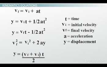
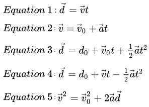
There are four main kinematic equations that are commonly used in physics. These equations relate the displacement (Δx), initial velocity (v₀), final velocity (v), acceleration (a), and time (t) of an object moving in a straight line. The equations are as follows:
- Equation 1: (Δx = v₀t + frac{1}{2}at²)
- Equation 2: (v = v₀ + at)
- Equation 3: (v² = v₀² + 2aΔx)
- Equation 4: (Δx = frac{(v + v₀)t}{2})
These equations can be used to solve a variety of problems, such as finding the displacement of an object given its initial velocity, acceleration, and time. They can also be used to find the final velocity of an object given its initial velocity, acceleration, and displacement. Additionally, they can be used to find the time required for an object to reach a certain displacement or velocity.
It is important to note that these equations only apply to motion in a straight line with constant acceleration. If the acceleration is not constant, or if the motion involves other factors such as rotation or curved paths, different equations or techniques may be required.
Displacement Equations
The concept of displacement is an important one in physics, particularly in the study of kinematics. Displacement refers to the change in position of an object from its initial location to its final location. It is a vector quantity, meaning that it has both magnitude and direction. Displacement is typically represented by the symbol Δx.
There are several equations that can be used to calculate displacement in different scenarios. The specific equation to use depends on the information that is known about the object’s motion. One of the most basic displacement equations is:
Δx = xf – xi
This equation calculates displacement by subtracting the initial position (xi) from the final position (xf). The result is the change in position, or displacement, of the object.
Another displacement equation is:
Δx = v0t + 0.5at^2
This equation is often used when an object is undergoing constant acceleration. It takes into account the initial velocity (v0), the time (t), and the acceleration (a) of the object to calculate the displacement.
These are just two examples of displacement equations, and there are many more that can be used depending on the specific conditions of the motion. Understanding and using displacement equations is essential for accurately describing and analyzing the motion of objects in physics.
Velocity Equations
The velocity of an object is a measure of how quickly it changes its position. In physics, velocity is a vector quantity, meaning it has both magnitude and direction. To calculate the velocity of an object, we use velocity equations that relate the change in position, time, and acceleration.
There are several velocity equations that can be used in different situations. One of the most basic ones is the average velocity equation, which is given by:
Average Velocity = Change in Position / Change in Time
This equation calculates the average velocity over a certain period of time. However, objects often have changing velocities, so we need equations that can account for this. One such equation is the equation of motion, which relates the final velocity, initial velocity, acceleration, and time:
Final Velocity = Initial Velocity + (Acceleration x Time)
These velocity equations are fundamental tools in kinematics, the study of motion. By using these equations, we can accurately describe and predict the motion of objects in various scenarios.
Acceleration Equations

Acceleration is a fundamental concept in physics that measures how quickly the velocity of an object changes. It is defined as the rate at which an object’s velocity changes over time. Just as there are equations to describe the motion of an object, there are also equations to describe the acceleration of an object.
One of the most basic acceleration equations is the kinematic equation for acceleration, which relates an object’s final velocity, initial velocity, acceleration, and time. This equation is represented as:
v = u + at
Where v represents the final velocity, u represents the initial velocity, a represents the acceleration, and t represents the time.
Another important equation is the equation that relates an object’s velocity and displacement to its acceleration. This equation is represented as:
v^2 = u^2 + 2as
Where s represents the displacement.
These equations are incredibly useful in physics as they allow us to calculate the acceleration of an object based on its initial and final velocities, displacement, and time. By understanding these equations, we can analyze and predict the motion of objects in various scenarios.
How to Solve Kinematic Equations Worksheets
When it comes to solving kinematic equations worksheets, it’s important to have a clear understanding of the concepts involved. Kinematic equations describe the motion of objects and can be used to solve various problems related to displacement, velocity, acceleration, and time.
Here are some steps to help you solve kinematic equations worksheets:
- Identify the given information: Read through the problem carefully and identify the information provided. This usually includes values such as initial velocity, final velocity, acceleration, time, and displacement.
- Choose the appropriate equation: Based on the given information and what you are asked to solve for, choose the kinematic equation that is most relevant to the problem.
- Plug in the known values: Substitute the known values into the chosen kinematic equation. Make sure to pay attention to units and use consistent units throughout the calculation.
- Solve for the unknown: Rearrange the equation to solve for the unknown variable. It may be necessary to use algebraic manipulation to isolate the variable.
- Check your answer: Once you have calculated the unknown variable, double-check your work to ensure that it makes sense in the context of the problem. If applicable, compare your answer to the given values to verify its accuracy.
By following these steps and practicing solving kinematic equations worksheets, you can improve your understanding of kinematics and develop problem-solving skills in physics.
Step-by-Step Guide to Solving Kinematic Equations
When solving kinematic equations, it is important to follow a systematic approach to ensure proper calculation and understanding of the problem at hand. By following a step-by-step guide, you can minimize errors and confidently solve for various kinematic quantities.
Step 1: Identify Known and Unknown Variables
Start by identifying the variables given in the problem and the variables you need to solve for. These variables include displacement (Δx), initial velocity (v0), final velocity (v), acceleration (a), and time (t).
Step 2: Choose the Appropriate Kinematic Equation
Based on the known and unknown variables, select the appropriate kinematic equation to use. The four main kinematic equations are:
- Equation 1: Δx = v0t + 0.5at^2
- Equation 2: v = v0 + at
- Equation 3: v^2 = v0^2 + 2aΔx
- Equation 4: Δx = 0.5(v0 + v)t
Choose the equation that contains the known variables and will allow you to solve for the desired unknown variable.
Step 3: Substitute Given Values and Solve
Substitute the known values into the selected equation and solve for the unknown variable. Make sure to always use consistent units for all variables to avoid errors in calculation.
Step 4: Check your Answer
Once you have obtained the solution, double-check your answer by substituting the calculated values back into the original equation. This will help verify the accuracy of your calculations.
By following this step-by-step guide, you can confidently solve kinematic equations and accurately determine important quantities related to motion. Practice and familiarity with different scenarios will improve your ability to solve these equations effectively.