
Graphing logarithmic functions is an important skill in mathematics, as it allows us to visualize and understand the behavior of these functions. In this article, we will explore the topic of graphing logarithmic functions and provide answers to the exercise 15 2 on this subject.
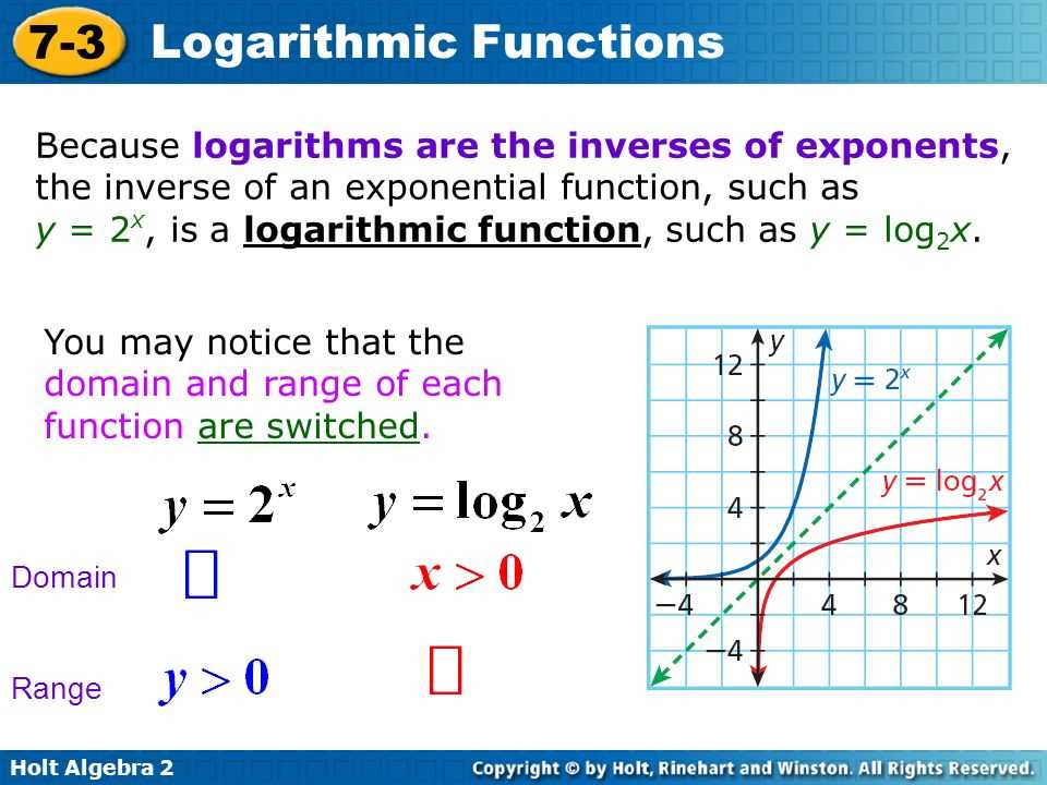
A logarithmic function is the inverse of an exponential function. It is represented by the equation y = log(base a) x, where a is the base of the logarithm and x is the input value. The graph of a logarithmic function will have a specific shape depending on the value of the base.
In exercise 15 2, we are given a set of logarithmic functions and are asked to graph them. By using the properties and rules of logarithmic functions, we can determine the behavior of these functions and plot their graphs on a coordinate plane. The answers to exercise 15 2 will provide us with a visual representation of how these functions behave and intersect with the x and y axes.
Understanding how to graph logarithmic functions is an essential skill for solving various mathematical problems and analyzing real-world phenomena. By studying and practicing exercises like 15 2, we can develop a strong understanding of logarithmic functions and their graphical representations. With these skills, we can accurately analyze and interpret data in various fields, including finance, physics, and biology.
What is a logarithmic function?
A logarithmic function is a mathematical function that represents the inverse of an exponential function. In other words, it is the function that relates a given logarithm to its base. Logarithmic functions are commonly denoted as logb(x), where b is the base and x is the argument of the logarithm.
Logarithmic functions have various properties that make them useful in many mathematical and scientific applications. One of the key properties is that logarithms can be used to solve exponential equations. By applying logarithmic functions, exponential equations can be transformed into more manageable forms.
Logarithmic functions also have a distinct shape when graphed. The graph of a logarithmic function is a smooth curve that increases or decreases slowly and approaches a vertical asymptote. The behavior of the graph depends on the value of the base. For example, if the base is greater than 1, the graph will increase as the argument increases. If the base is between 0 and 1, the graph will decrease as the argument increases.
Overall, logarithmic functions are powerful tools in mathematics and various fields of science. They allow for the efficient representation and manipulation of exponential relationships, making them indispensable in solving complex equations and analyzing data.
How to graph a logarithmic function?
Graphing a logarithmic function involves several steps to accurately plot the points and sketch the curve. Here is a step-by-step guide on how to graph a logarithmic function:
Step 1: Identify the base and the domain
The first step is to determine the base of the logarithmic function. It is typically denoted as “log base b,” where b represents a positive number greater than 1. Next, identify the domain of the function, which is the set of all possible x-values for the function.
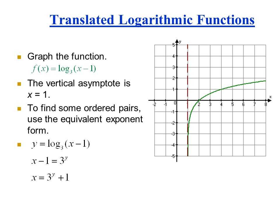
Step 2: Find the vertical asymptote
In a logarithmic function, the vertical asymptote occurs when the log expression is undefined. To find the vertical asymptote, set the argument of the logarithm equal to zero and solve for the x-value.
Step 3: Determine the transformations
Logarithmic functions can undergo transformations such as vertical shifts, horizontal shifts, and vertical stretches or compressions. Analyze the equation of the function to determine if any transformations are present and note the direction and amount of each transformation.
Step 4: Plot key points
Choose a few x-values within the domain and evaluate the logarithmic function to find the corresponding y-values. Plot these key points on the graph.
Step 5: Sketch the curve
Connect the plotted points to create a smooth curve that represents the logarithmic function. Pay attention to the asymptote, transformations, and overall shape of the graph.
By following these steps, you can accurately graph a logarithmic function and visualize its behavior and characteristics.
Understanding the domain and range of logarithmic functions
Logarithmic functions are a type of mathematical function that involve the logarithm of a number. These functions can be represented graphically, and understanding their domain and range is essential for properly interpreting and analyzing the graphs. The domain of a logarithmic function is the set of all possible input values, while the range is the set of all possible output values.
When graphing logarithmic functions, it is important to note that the domain is restricted to positive input values. This is because the logarithm of a negative number or zero is undefined. Therefore, the domain of a logarithmic function is typically expressed as x > 0. It is also possible to have an additional restriction on the domain, such as x ≠ 1, to avoid an undefined value at the logarithm base.
The range of a logarithmic function is the set of all possible output values. For logarithmic functions, the range is typically expressed as all real numbers, or (-∞, ∞). This is because the logarithmic function can produce any real number as its output. However, it’s important to consider any additional restrictions that may be imposed by the specific logarithmic function being graphed.
In summary, when graphing logarithmic functions, it is crucial to understand that the domain is restricted to positive input values and possibly other restrictions, while the range is typically all real numbers. By understanding the domain and range of logarithmic functions, we can accurately interpret and analyze their graphs to gain insights into various mathematical and real-world problems.
Solving logarithmic equations
Logarithmic equations involve solving for the unknown variable within a logarithmic function. These equations typically require logarithmic properties and rules to simplify and solve them. Here are some steps to solve logarithmic equations:
- Step 1: Determine the domain of the logarithmic function to identify any restrictions on the variable. The argument of a logarithm must be greater than zero.
- Step 2: Apply logarithmic properties to simplify the equation. These properties include the product rule, quotient rule, and power rule of logarithms.
- Step 3: Isolate the logarithmic expression by moving any other terms to the opposite side of the equation.
- Step 4: Convert the equation into exponential form if possible. This allows for easier solving by matching bases.
- Step 5: Solve for the variable using algebraic techniques such as factoring, completing the square, or using the quadratic formula if necessary.
- Step 6: Check the solution(s) obtained by substituting them back into the original equation. It is important to verify that the solution(s) satisfy the domain restrictions.
Solving logarithmic equations can require a combination of algebraic manipulations, logarithmic properties, and solving techniques. It is important to understand these steps and practice applying them to different types of logarithmic equations.
The properties of logarithmic functions

Logarithmic functions are a special type of mathematical function that involve the logarithm of a given number. These functions have several properties that make them unique and useful in various applications. One important property is that the logarithm of a product of two numbers is equal to the sum of the logarithms of the individual numbers. This property is known as the product rule for logarithms and can be expressed as:
logb(xy) = logb(x) + logb(y)
Another property of logarithmic functions is the power rule. According to this rule, the logarithm of a number raised to a power is equal to the product of the power and the logarithm of the number. Mathematically, it can be written as:
logb(xn) = n * logb(x)
Logarithmic functions also possess the property of the change of base. This property allows us to convert logarithms from one base to another. The formula for the change of base can be expressed as:
| logb(x) | = | loga(x) / loga(b) |
|---|
These properties of logarithmic functions are fundamental in solving logarithmic equations and simplifying complex mathematical expressions. They play a crucial role in various fields such as mathematics, engineering, finance, and computer science.
Transformations of logarithmic functions
Logarithmic functions can be transformed in various ways to change their shape and position on a graph. These transformations allow us to manipulate the behavior of the function and adapt it to different contexts and purposes.
One common transformation is a vertical shift, which moves the entire graph up or down. A positive vertical shift shifts the graph upward, while a negative shift moves it downward. The amount of the shift is determined by the value added or subtracted to the function’s equation.
An additional transformation is a horizontal shift, which moves the graph left or right. A positive horizontal shift shifts the graph to the right, while a negative shift moves it to the left. This shift is determined by the value added or subtracted inside the logarithmic function’s argument.
Another transformation is a vertical stretch or compression, which changes the vertical scale of the graph. A vertical stretch expands the graph vertically, making it appear narrower, while a compression makes it appear wider. This transformation is achieved by multiplying the function’s equation by a constant greater than 1 for stretching or less than 1 for compression.
A final transformation is a reflection in the x-axis, which flips the graph upside down. This can be achieved by multiplying the function’s equation by -1. The reflection changes the sign of the entire function.
By combining these transformations, we can create complex logarithmic functions that exhibit various behaviors and characteristics. It is important to understand how each transformation affects the graph to accurately represent and interpret logarithmic functions in different situations.
Applications of Logarithmic Functions
Logarithmic functions have numerous applications in various fields, including mathematics, science, economics, and engineering. They are particularly useful when dealing with exponential growth or decay situations and when analyzing data that spans a large range of values.
In mathematics, logarithmic functions are commonly used to solve equations involving exponential growth or decay. They allow us to determine the time or amount required for a quantity to reach a certain value. Logarithms also play a crucial role in calculus, where they are used to simplify calculations and solve complex equations.
In science, logarithmic functions are used to describe the intensity of earthquakes, the pH level of a solution, the rate of radioactive decay, and the sound or light intensity. They help scientists analyze and interpret data that have exponential relationships, such as population growth, enzyme reactions, or the concentration of substances over time.
In economics, logarithmic functions are employed to model and analyze a wide range of phenomena, including compound interest, inflation rates, and stock market fluctuations. They are particularly useful in financial calculations, where exponential growth or decay is common, such as in compound interest calculations or evaluating investment returns.
In engineering, logarithmic functions are extensively used in various applications, such as signal processing, telecommunications, and control systems. They help engineers analyze and design systems with exponential response characteristics, such as amplifiers, filters, or feedback loops.
Overall, logarithmic functions are a powerful tool that allows researchers, scientists, mathematicians, and engineers to describe and analyze exponential phenomena, model complex systems, and make predictions based on data with exponential relationships. Their applications are diverse and essential in various fields of study and industry.
Common mistakes when graphing logarithmic functions
Graphing logarithmic functions can be a challenging task for students, and it is not uncommon for them to make mistakes along the way. Understanding these common mistakes can help students improve their graphing skills and avoid errors. Here are some common mistakes to watch out for:
- Incorrectly identifying the vertical asymptote: One common mistake is incorrectly identifying the vertical asymptote of the logarithmic function. The vertical asymptote is located at x = a, where a is the value inside the logarithmic function’s argument. Students may mistakenly identify the vertical asymptote at x = a+1 or x = a-1, leading to incorrect graphing.
- Errors in plotting the points: Another common mistake is making errors in plotting the points on the graph. It is important to accurately calculate the values of the logarithmic function for different x-values and plot them correctly on the graph. Small calculation errors or inaccuracies can result in a completely different graph.
- Ignoring the domain and range: Many students overlook the domain and range restrictions of logarithmic functions. Logarithmic functions have specific domain and range values that must be considered when graphing. Ignoring these restrictions can lead to graphing errors and inaccurate representations of the function.
- Confusing the shape of the graph: The shape of logarithmic functions is often misunderstood by students. Some may mistakenly think that logarithmic functions have a linear shape, while others may confuse it with an exponential curve. Understanding the correct shape of the graph is crucial in accurately representing the function.
- Forgetting the base: Logarithmic functions have a base value that should not be overlooked. Forgetting to include the base value can result in an incorrect graph and inaccurate representation of the function.
Avoiding these common mistakes and developing a solid understanding of the properties of logarithmic functions can greatly improve a student’s ability to graph them accurately. Practice and attention to detail are key in mastering graphing logarithmic functions.