
Understanding how to graph cube root functions is an essential skill in mathematics. Whether you’re a student or a teacher, being able to solve problems involving cube root functions is key to mastering this area of study. In this article, we will explore a series of practice problems, along with their corresponding answers, to help you sharpen your graphing skills.
First, let’s review the basics of cube root functions. A cube root function is a type of radical function where the variable is raised to the power of one-third. The graph of a cube root function is a curve that starts at the origin and extends through the positive and negative quadrants. Understanding the shape of this curve is crucial for accurately graphing these functions.
Now, let’s dive into the practice problems. We will provide five different equations, and your task is to graph each function on a coordinate plane. Pay close attention to the domain and range of each function, as well as the intercepts, asymptotes, and any other key features. To help you check your work, we will also provide the answer key for each problem.
By practicing graphing cube root functions, you will gain a deeper understanding of their properties and characteristics. This will enable you to confidently solve more complex problems involving cube root functions in the future. So, let’s get started and sharpen our skills in graphing cube root functions!
Overview of Cube Root Functions
Cube root functions are a type of radical function that involve taking the cube root of a variable. The cube root of a number x is the number y such that y^3 = x. Cube root functions are written in the form f(x) = ∛x, where the cube root symbol (∛) indicates that the function takes the cube root of the variable x.
Cube root functions have a unique shape that sets them apart from other types of functions. When graphed, cube root functions form a curve that starts at the origin (0,0) and extends off into the positive and negative x and y directions. The curve is similar in shape to a parabola, but it is flatter and wider. The curve approaches the x-axis and y-axis, but never intersects them.
Cube root functions can have both positive and negative outputs for a given input. This is because the cube root of a positive number can be both positive and negative, while the cube root of a negative number is always negative. As a result, the graph of a cube root function will have both positive and negative branches that mirror each other symmetrically along the y-axis.
Cube root functions are commonly used in mathematics and science to model various phenomena. They can be used to describe the relationship between a variable and its cube root, such as in growth and decay problems or in measuring the volume of a cube. Understanding the properties and graph of cube root functions is important for analyzing and solving problems involving cube root functions.
What is a Cube Root Function?
A cube root function is a type of mathematical function that involves finding the cube root of a given variable or expression. It can be represented in the form f(x) = ∛x, where ∛ represents the cube root operation.
The cube root of a number x is the value that, when raised to the power of 3, gives the original number. For example, the cube root of 8 is 2 because 2^3 = 8. Similarly, the cube root of -27 is -3 because -3^3 = -27.
Cube root functions can be graphed on a coordinate plane, where the x-axis represents the input values and the y-axis represents the corresponding output values. The graph of a cube root function has a characteristic shape, known as an S-shaped curve, due to the nature of the cube root operation.
- When x is positive, the corresponding y-values are also positive, resulting in the upward-sloping portion of the curve.
- When x is negative, the corresponding y-values are negative, resulting in the downward-sloping portion of the curve.
- The graph of the cube root function passes through the origin (0, 0).
Understanding cube root functions is important in various fields of study, including mathematics, engineering, and physics. They are used to solve equations, model real-world phenomena, and analyze the behavior of certain systems. By studying cube root functions, mathematicians and scientists gain insights into the relationships between variables and the properties of numbers.
Properties of Cube Root Functions
Cube root functions are a specific type of radical function, where the variable is taken to the power of $frac{1}{3}$. These functions have several notable properties that distinguish them from other types of functions.
1. Domain and Range: The domain of a cube root function is all real numbers, because the cube root can be taken of any real number. The range, however, may be limited depending on the function’s equation. For example, the cube root function $y = sqrt[3]{x}$ has a range of all real numbers, while the cube root function $y = -sqrt[3]{x}$ has a range of all negative real numbers.
2. Symmetry: Cube root functions are typically symmetric with respect to the origin (0,0). This means that if you reflect the graph of the function across the x-axis and y-axis, it will remain unchanged. This symmetry can be observed in the shape of the graph, which is similar to an inverted cubic parabola.
3. Intercepts: The cube root function $y = sqrt[3]{x}$ has the x-intercept at (0,0), because $sqrt[3]{0} = 0$. The y-intercept, however, does not exist because there is no value of x that will result in a y-value of 0.
4. Increasing/Decreasing: Cube root functions are increasing for positive values of x, and decreasing for negative values of x. This can be observed in the graph of the function, where the curve starts at the origin and moves upwards for positive x-values, and downwards for negative x-values.
Overall, cube root functions have distinct characteristics that make them unique among other types of functions. Understanding these properties is essential for analyzing and graphing cube root functions accurately.
How to Graph Cube Root Functions
If you’re studying graphing functions, it’s important to understand how to graph cube root functions. A cube root function is a type of radical function in which the input variable is raised to the power of one-third. To graph a cube root function, follow these steps:
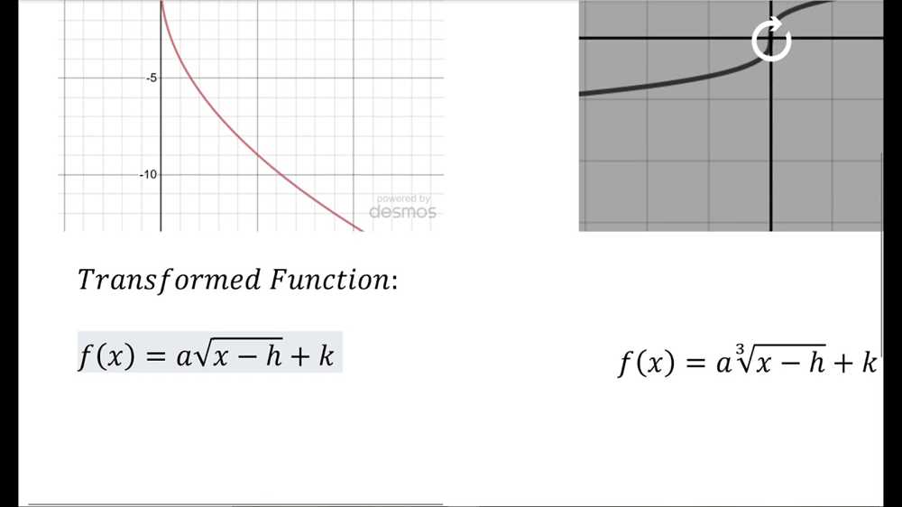
- Identify the parent function: The parent function of a cube root function is f(x) = ∛x. This function has a domain of all real numbers and a range of all real numbers. The graph of the parent function passes through the point (0, 0).
- Determine the transformations: Cube root functions can be transformed by shifting, stretching, or compressing the graph. The transformations can be described using the following functions: f(x) = a∛(b(x – h)) + k. The values of a, b, h, and k determine the transformations on the graph.
- Plot the key points: To graph the function, choose some x-values and calculate the corresponding y-values using the function equation. Some key points to plot include the intercepts (when f(x) = 0), the vertex (the highest or lowest point on the graph), and any additional points to help determine the shape of the graph.
- Draw the graph: Connect the plotted points with a smooth curve. Keep in mind the shape of a cube root function, which is similar to a half of a sideways parabola. Extend the graph as necessary to show the domain and range of the function.
By following these steps, you can graph cube root functions and better understand their behavior. Practice graphing different cube root functions to improve your skills and deepen your understanding of this important mathematical concept.
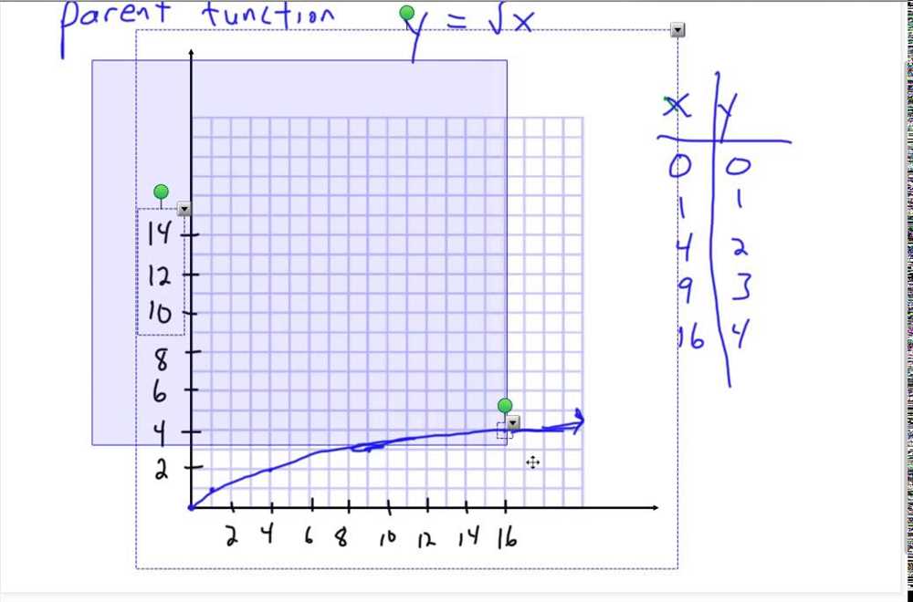
Examining the Parent Function
The cube root function is an important type of function that can be used to model various real-life situations. It is represented by the equation y = ∛x, where x is the input and y is the output. The cube root function is a special case of the more general power function, where the exponent is 1/3. This specific exponent results in the function having both positive and negative outputs, making it a unique and interesting function to study.
When examining the parent function of y = ∛x, it is important to understand its key characteristics. One of the most notable features is that its graph passes through the origin (0,0). This means that when x is 0, the output y will also be 0. Additionally, the parent function is symmetric about the origin, which means that it is reflective across both the x and y axes.
Looking at the graph of the cube root function, it is clear that the function has a gentle, curved shape. As x increases, the graph becomes steeper, indicating that the rate of change of y with respect to x is increasing. On the other hand, as x decreases, the graph becomes less steep, showing a decreasing rate of change. This is because the cube root function is a non-linear function, meaning that its rate of change is not constant.
Overall, examining the parent function of y = ∛x can provide insight into the behavior of this particular type of function. From its symmetric nature to its changing rate of change, understanding the characteristics of the cube root function is essential for further analyzing and manipulating it in mathematical and practical applications.
Identifying Key Points and Plotting the Graph
When graphing cube root functions, it is important to identify key points that will help in plotting the graph accurately. A cube root function is of the form f(x) = ∛x, where the cube root of a number x is the value that, when raised to the power of 3, gives the number x. In other words, f(x) is equal to the number that, when cubed, produces x.
One key point to identify is the x-intercept, which is the point at which the graph crosses the x-axis. For a cube root function, the x-intercept is (0, 0), since the cube root of 0 is 0. This is the point where the graph starts.
Another key point to identify is the y-intercept, which is the point at which the graph crosses the y-axis. For a cube root function, the y-intercept is also (0, 0), since the cube root of 0 is 0. This means that the graph passes through the origin.
Other key points can be identified by choosing different values of x and finding the corresponding values of f(x). For example, if we choose x = 1, then f(1) = ∛1 = 1. So, the point (1, 1) is on the graph. Similarly, if we choose x = 8, then f(8) = ∛8 = 2. So, the point (8, 2) is on the graph.
Once the key points are identified, they can be plotted on a graph and connected to create the graph of the cube root function. By using additional points and connecting them smoothly, we can get a better understanding of the shape of the graph and any other key features it may possess.
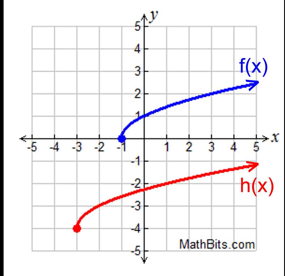
Examples of Graphing Cube Root Functions
Cube root functions represent a type of mathematical function that involves taking the cube root of a variable. These types of functions are often used in analytical geometry and can be represented graphically to visualize their behavior.
Let’s consider some examples of graphing cube root functions:
Example 1:

Graph the function f(x) = ³√x.
To graph this function, we can choose different values for x and calculate the corresponding y-values by taking the cube root of x. For example, when x = 1, y = ³√1 = 1. When x = 8, y = ³√8 = 2. Therefore, we plot the points (1, 1) and (8, 2) on the graph. By connecting these points, we can observe that the graph of f(x) = ³√x is a curve that passes through the origin and steadily increases as x increases.
Example 2:
Graph the function g(x) = -³√x.
In this example, the function is multiplied by -1, which reflects the graph across the x-axis. By applying the same approach as Example 1, we can plot points such as (1, -1) and (8, -2). Connecting these points results in a curve that starts from the origin and steadily decreases as x increases.
These examples demonstrate how graphing cube root functions can help visualize the relationship between the input variable x and the output variable y. By plotting various points and connecting them, we can understand the behavior of the function and its characteristics, such as symmetry or steepness. Understanding these graphs can be useful in solving equations involving cube root functions or analyzing real-world situations where cube root functions may be applicable.
Common Mistakes to Avoid when Graphing Cube Root Functions
When graphing cube root functions, it is important to be aware of some common mistakes that students often make. These mistakes can lead to inaccuracies or incorrect representations of the functions. By understanding and avoiding these mistakes, students can ensure that their graphs are accurate and precise.
1. Forgetting to consider the domain: Cube root functions have a restricted domain, meaning that not all values of x are valid inputs. It is crucial to determine the appropriate domain for the function and only plot points within that domain. Forgetting to consider the domain can result in inaccurate graphs.
2. Incorrectly identifying the end behavior: Cube root functions have a specific end behavior, which means that as x approaches positive or negative infinity, the function approaches positive or negative infinity, respectively. Failing to identify and correctly represent this end behavior can lead to an incorrect graph.
3. Misinterpreting the shape of the graph: Cube root functions have a distinct shape, resembling the letter “S”. Students sometimes mistakenly graph a straight line or a different curve instead of the proper shape. It is essential to understand the unique shape of cube root functions to accurately represent them on a graph.
4. Ignoring the x-intercepts: Cube root functions often have x-intercepts, where the function crosses the x-axis. Ignoring or incorrectly identifying these x-intercepts can result in an inaccurate graph. It is important to locate and plot the x-intercepts correctly for an accurate representation of the function.
5. Not labeling the axes and points: Graphs should always be properly labeled, including the x and y axes. It is also essential to label any significant points, such as the x-intercepts or any points of interest. Failing to label the axes and points can make the graph confusing and difficult to interpret.
In summary, when graphing cube root functions, it is crucial to consider the domain, correctly identify the end behavior, interpret the shape of the graph accurately, locate and label the x-intercepts, and properly label the axes and points. By avoiding these common mistakes, students can create precise and accurate graphs of cube root functions.