
The normal distribution is one of the most important concepts in statistics and probability theory. It is a continuous probability distribution that is symmetric and bell-shaped. Understanding the properties of the normal distribution is crucial for many statistical analyses and hypothesis testing.
A normal distribution worksheet is a valuable tool for practicing and assessing one’s understanding of the normal distribution. It typically consists of a series of questions and exercises related to various concepts and calculations associated with the normal distribution. These worksheets are designed to help students gain proficiency in solving problems involving mean, standard deviation, z-scores, and probability calculations.
This article presents a normal distribution worksheet with answers, which provides a step-by-step solution to each problem and a brief explanation of the underlying concepts. It is a valuable resource for students, teachers, and anyone interested in learning and practicing the normal distribution. The worksheet covers a range of topics, including finding probabilities for specific values, calculating z-scores, and determining percentiles in a normal distribution.
By working through the normal distribution worksheet with answers, students can enhance their understanding of the normal distribution, develop problem-solving skills, and gain confidence in their ability to analyze and interpret data using this fundamental statistical concept.
What is Normal Distribution?
Normal distribution, also known as Gaussian distribution or bell curve, is one of the most important concepts in statistics. It is a continuous probability distribution characterized by a symmetric bell-shaped curve.
The key features of a normal distribution are its mean (μ) and standard deviation (σ), which determine the shape, location, and spread of the curve. The mean represents the center or average value of the data, while the standard deviation measures how spread out the data is from the mean.
In a normal distribution, the curve is symmetrical around the mean. This means that approximately 50% of the data falls on either side of the mean, and the remaining 50% is distributed evenly on both tails of the curve. The curve is bell-shaped, with the highest point at the mean, and it extends to negative and positive infinity on both ends.
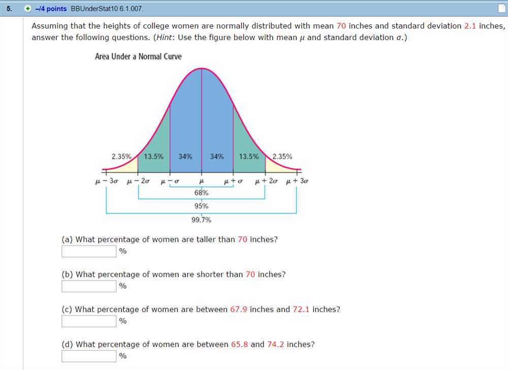
The standard deviation plays a crucial role in normal distribution. It determines the spread of the data and helps us understand the variability or dispersion of the values. In a standard normal distribution, where the mean is zero and the standard deviation is one, about 68% of the data falls within one standard deviation of the mean, 95% falls within two standard deviations, and 99.7% falls within three standard deviations.
Normal distribution is widely used in various fields such as economics, biology, psychology, and quality control. It provides a foundation for many statistical analyses and helps us make predictions and draw conclusions based on data.
Let’s summarize the key points:
- Normal distribution is a continuous probability distribution characterized by a symmetric bell-shaped curve.
- The mean represents the center of the data, while the standard deviation measures the spread.
- The curve is symmetrical around the mean, with approximately 50% of the data falling on either side.
- The standard deviation determines the spread and helps understand the variability of the values.
- Normal distribution is widely used in various fields and provides a foundation for statistical analysis.
Definition and Characteristics

One of the key characteristics of a normal distribution is its bell shape. The curve is symmetric, meaning that the left half and the right half of the curve are mirror images of each other. This symmetry indicates that the probabilities of values occurring on one side of the mean are equal to the probabilities of values occurring on the other side of the mean.
Another important characteristic of a normal distribution is that it is continuous. This means that there are an infinite number of possible values that can be observed within the distribution. Unlike discrete distributions, which are characterized by distinct values, a normal distribution allows for any possible value within a given range.
The mean of a normal distribution is located at the center of the curve, representing the average value of the data. The standard deviation measures the dispersion of the values around the mean. It provides an indication of how spread out the data points are and is used to calculate the probabilities of observing values within specific ranges.
The normal distribution is widely used in statistics and data analysis due to its mathematical properties and its tendency to fit many phenomena in nature, such as heights, weights, test scores, and IQ scores. It serves as a useful model for describing and analyzing data, allowing researchers to make predictions and draw conclusions based on the assumptions of normality.
In conclusion, a normal distribution is a symmetrical probability distribution that follows a bell-shaped curve. It is characterized by its bell shape, continuity, mean, and standard deviation. It is commonly used in statistics to describe and analyze real-world data.
Properties and Uses
The normal distribution, also known as the Gaussian distribution, is a probability distribution that is widely used in statistics and various fields of science. It is characterized by its bell-shaped curve, with the majority of the data falling around the mean and decreasing symmetrically towards the tails.
One of the important properties of the normal distribution is its symmetry. The mean, median, and mode of a normal distribution are all equal, making it a convenient choice for many statistical analyses. Additionally, the distribution is fully characterized by two parameters – the mean and the standard deviation. This allows for easy interpretation and comparison of data across different normal distributions.
The normal distribution has various uses in practice. It is often used in hypothesis testing, where researchers compare observed data to a theoretical normal distribution to determine the likelihood of chance variations. In addition, many statistical tests and confidence intervals assume that the data come from a normal distribution. This assumption simplifies the calculations and allows for more accurate results. Furthermore, the normal distribution is commonly used in quality control processes, where it helps in identifying deviations from a standard or target value. Its symmetric properties and known probabilities make it a valuable tool for decision-making and risk analysis.
Overall, the normal distribution is a powerful mathematical concept that provides a simple and convenient way to model and analyze real-world data. Its properties and uses make it a fundamental tool in statistics and various scientific disciplines, enabling researchers and practitioners to make informed decisions and draw reliable conclusions.
How to Create a Normal Distribution Worksheet
Creating a normal distribution worksheet is a great way to help students understand the concept of normal distribution and practice solving problems related to it. In order to create an effective worksheet, there are several key steps to follow.
Step 1: Define the Basics
- Start by introducing the concept of normal distribution and explaining its characteristics.
- Define key terms such as mean, standard deviation, and z-score.
- Provide examples or real-life scenarios to illustrate the application of normal distribution.
Step 2: Include Practice Problems
- Include a variety of practice problems that cover different aspects of normal distribution.
- Start with easier problems that involve finding probabilities or areas under the curve.
- Gradually increase the difficulty level by including problems that require using z-scores or solving for specific values.
- Provide step-by-step solutions for each problem to guide students through the process.
Step 3: Include Application Questions
- Include application questions that require students to analyze and interpret real-world data using normal distribution.
- Use examples from various fields such as finance, biology, or psychology to make the questions more relatable and engaging.
- Encourage students to explain their reasoning and think critically about the results.
Step 4: Include Graphical Representations
- Incorporate graphical representations of normal distribution, such as histograms or bell curves, to visually reinforce the concept.
- Give students opportunities to practice interpreting and analyzing the graphs.
- Provide clear explanations and labels for all the components of the graph.
By following these steps, you can create a comprehensive and effective normal distribution worksheet that will help students develop a solid understanding of the topic and improve their problem-solving skills.
Steps and Guidelines

When working with a normal distribution worksheet, it is important to follow a set of steps and guidelines in order to properly analyze and solve the given problems. These steps and guidelines can help ensure accuracy and efficiency in your calculations.
To begin with, it is essential to understand the concept of a normal distribution and its characteristics. A normal distribution is a continuous probability distribution that is symmetric and bell-shaped. It is characterized by its mean and standard deviation, which determine the center and spread of the distribution.
Once you have a clear understanding of the normal distribution, you can follow the following steps and guidelines:
- Identify the problem: Read the problem carefully and identify the information given, such as the mean, standard deviation, and any specific requirements or conditions.
- Draw a normal distribution curve: Use a graph or a diagram to represent the normal distribution curve, labeling the mean and marking any specific values or intervals mentioned in the problem.
- Calculate probabilities: Use the standard normal distribution table or a calculator to find the probabilities associated with specific values or intervals. Convert the given values to z-scores using the formula (x – mean) / standard deviation.
- Apply the empirical rule or the central limit theorem: If the problem involves a large sample size or a proportion, you can use the empirical rule or the central limit theorem to estimate probabilities.
- Interpret the results: Finally, interpret the calculated probabilities in the context of the problem, making sure to answer any specific questions or requirements.
By following these steps and guidelines, you can effectively solve problems related to normal distributions and accurately analyze the given data. Practice and familiarity with these concepts will also help improve your problem-solving skills in this area.
Example Problems
Here are a few example problems to help you practice working with normal distribution:
Problem 1:
A company manufactures light bulbs, and the lifespan of the bulbs is normally distributed with a mean of 800 hours and a standard deviation of 50 hours. What is the probability that a randomly selected light bulb will last between 750 and 850 hours?
Solution: To solve this problem, we need to find the area under the normal curve between 750 hours and 850 hours. We can use the z-score formula to standardize the values for calculation. The z-score for 750 hours is (750 – 800) / 50 = -1, and the z-score for 850 hours is (850 – 800) / 50 = 1. Using a z-table or calculator, we can find the probabilities associated with these z-scores. The probability of a random light bulb lasting between 750 and 850 hours is the difference between the probabilities corresponding to -1 and 1 on the z-table.
Problem 2:
The heights of male students at a certain college are normally distributed with a mean of 70 inches and a standard deviation of 3 inches. What is the probability that a randomly selected male student is taller than 75 inches?
Solution: To solve this problem, we need to find the area under the normal curve to the right of 75 inches. We can use the z-score formula to standardize the value for calculation. The z-score for 75 inches is (75 – 70) / 3 = 1.67. Using a z-table or calculator, we can find the probability associated with this z-score. The probability of a randomly selected male student being taller than 75 inches is the area to the right of 1.67 on the z-table.
Problem 3:
The scores on a standardized test are normally distributed with a mean of 500 and a standard deviation of 100. What is the minimum score needed to be in the top 10% of test takers?
Solution: To solve this problem, we need to find the score that corresponds to the top 10% of test takers. We can use the z-score formula to find the z-score associated with the top 10% probability. The z-score corresponding to a 10% probability is found by using the z-table or calculator. Once we have the z-score, we can use the formula z = (x – mean) / standard deviation to find the corresponding score x.
Normal Distribution Worksheet Questions
In this worksheet, you will practice solving problems related to the normal distribution. The normal distribution, also known as the Gaussian distribution or bell curve, is a continuous probability distribution that is symmetric about its mean. It is commonly used in statistics to model various real-world phenomena.
1. Question: The heights of adult males in a certain population follow a normal distribution with a mean of 175 cm and a standard deviation of 7 cm. What percentage of adult males are shorter than 165 cm?
To solve this problem, we can use the properties of the standard normal distribution. First, we need to calculate the z-score for a height of 165 cm using the formula z = (x – μ) / σ, where x is the height, μ is the mean, and σ is the standard deviation. Substituting the given values, we get z = (165 – 175) / 7 = -1.43. We can then use a standard normal distribution table or a calculator to find the cumulative probability associated with a z-score of -1.43. Converting the z-score to a percentage, we find that approximately 7.58% of adult males are shorter than 165 cm.
2. Question: The scores on a standardized test follow a normal distribution with a mean of 500 and a standard deviation of 100. What is the probability that a randomly selected student scores between 400 and 600?
To solve this problem, we need to calculate the z-scores for the lower and upper bounds of the given range. For a score of 400, the z-score is (400 – 500) / 100 = -1. Similarly, for a score of 600, the z-score is (600 – 500) / 100 = 1. We can then find the cumulative probabilities associated with these z-scores using a standard normal distribution table or a calculator. Finally, we subtract the cumulative probability corresponding to the lower bound from the cumulative probability corresponding to the upper bound to find the probability that a randomly selected student scores between 400 and 600. This can be represented as P(-1 < z < 1) = P(z < 1) - P(z < -1).
3. Question: The weights of a certain type of fruit follow a normal distribution with a mean of 150 grams and a standard deviation of 10 grams. If a random sample of 50 fruits is taken, what is the probability that the average weight of the sample is between 145 and 155 grams?
To solve this problem, we can use the properties of the sampling distribution of the sample mean. The sampling distribution of the sample mean follows a normal distribution with a mean equal to the population mean and a standard deviation equal to the population standard deviation divided by the square root of the sample size. In this case, the mean of the sampling distribution is 150 grams, and the standard deviation is 10 grams / √50 ≈ 1.414 grams. We can then proceed to calculate the z-scores for the lower and upper bounds of the given range and find the corresponding cumulative probabilities using a standard normal distribution table or a calculator. Finally, we subtract the cumulative probability corresponding to the lower bound from the cumulative probability corresponding to the upper bound to find the desired probability. This can be represented as P(-1.414 < z < 1.414) = P(z < 1.414) - P(z < -1.414).